Disjoint Set Union
This article discusses the data structure Disjoint Set Union or DSU. Often it is also called Union Find because of its two main operations.
This data structure provides the following capabilities. We are given several elements, each of which is a separate set. A DSU will have an operation to combine any two sets, and it will be able to tell in which set a specific element is. The classical version also introduces a third operation, it can create a set from a new element.
Thus the basic interface of this data structure consists of only three operations:
make_set(v)- creates a new set consisting of the new elementvunion_sets(a, b)- merges the two specified sets (the set in which the elementais located, and the set in which the elementbis located)find_set(v)- returns the representative (also called leader) of the set that contains the elementv. This representative is an element of its corresponding set. It is selected in each set by the data structure itself (and can change over time, namely afterunion_setscalls). This representative can be used to check if two elements are part of the same set or not.aandbare exactly in the same set, iffind_set(a) == find_set(b). Otherwise they are in different sets.
As described in more detail later, the data structure allows you to do each of these operations in almost $O(1)$ time on average.
Also in one of the subsections an alternative structure of a DSU is explained, which achieves a slower average complexity of $O(\log n)$, but can be more powerful than the regular DSU structure.
Build an efficient data structure
We will store the sets in the form of trees: each tree will correspond to one set. And the root of the tree will be the representative/leader of the set.
In the following image you can see the representation of such trees.
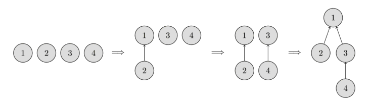
In the beginning, every element starts as a single set, therefore each vertex is its own tree. Then we combine the set containing the element 1 and the set containing the element 2. Then we combine the set containing the element 3 and the set containing the element 4. And in the last step, we combine the set containing the element 1 and the set containing the element 3.
For the implementation this means that we will have to maintain an array parent that stores a reference to its immediate ancestor in the tree.
Naive implementation
We can already write the first implementation of the Disjoint Set Union data structure. It will be pretty inefficient at first, but later we can improve it using two optimizations, so that it will take nearly constant time for each function call.
As we said, all the information about the sets of elements will be kept in an array parent.
To create a new set (operation make_set(v)), we simply create a tree with root in the vertex v, meaning that it is its own ancestor.
To combine two sets (operation union_sets(a, b)), we first find the representative of the set in which a is located, and the representative of the set in which b is located.
If the representatives are identical, that we have nothing to do, the sets are already merged.
Otherwise, we can simply specify that one of the representatives is the parent of the other representative - thereby combining the two trees.
Finally the implementation of the find representative function (operation find_set(v)):
we simply climb the ancestors of the vertex v until we reach the root, i.e. a vertex such that the reference to the ancestor leads to itself.
This operation is easily implemented recursively.
void make_set(int v) {
    parent[v] = v;
}

int find_set(int v) {
    if (v == parent[v])
        return v;
    return find_set(parent[v]);
}

void union_sets(int a, int b) {
    a = find_set(a);
    b = find_set(b);
    if (a != b)
        parent[b] = a;
}
However this implementation is inefficient.
It is easy to construct an example, so that the trees degenerate into long chains.
In that case each call find_set(v) can take $O(n)$ time.
This is far away from the complexity that we want to have (nearly constant time). Therefore we will consider two optimizations that will allow to significantly accelerate the work.
Path compression optimization
This optimization is designed for speeding up find_set.
If we call find_set(v) for some vertex v, we actually find the representative p for all vertices that we visit on the path between v and the actual representative p.
The trick is to make the paths for all those nodes shorter, by setting the parent of each visited vertex directly to p.
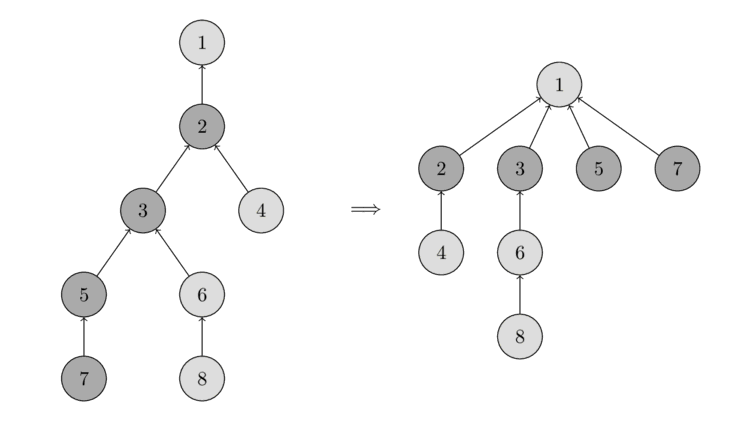
You can see the operation in the following image.
On the left there is a tree, and on the right side there is the compressed tree after calling find_set(7), which shortens the paths for the visited nodes 7, 5, 3 and 2.
The new implementation of find_set is as follows:
int find_set(int v) {
    if (v == parent[v])
        return v;
    return parent[v] = find_set(parent[v]);
}
The simple implementation does what was intended: first find the representative of the set (root vertex), and then in the process of stack unwinding the visited nodes are attached directly to the representative.
This simple modification of the operation already achieves the time complexity $O(\log n)$ per call on average (here without proof). There is a second modification, that will make it even faster.
Union by size / rank
In this optimization we will change the union_set operation.
To be precise, we will change which tree gets attached to the other one.
In the naive implementation the second tree always got attached to the first one.
In practice that can lead to trees containing chains of length $O(n)$.
With this optimization we will avoid this by choosing very carefully which tree gets attached.
There are many possible heuristics that can be used. Most popular are the following two approaches: In the first approach we use the size of the trees as rank, and in the second one we use the depth of the tree (more precisely, the upper bound on the tree depth, because the depth will get smaller when applying path compression).
In both approaches the essence of the optimization is the same: we attach the tree with the lower rank to the one with the bigger rank.
Here is the implementation of union by size:
void make_set(int v) {
    parent[v] = v;
    size[v] = 1;
}

void union_sets(int a, int b) {
    a = find_set(a);
    b = find_set(b);
    if (a != b) {
        if (size[a] < size[b])
            swap(a, b);
        parent[b] = a;
        size[a] += size[b];
    }
}
And here is the implementation of union by rank based on the depth of the trees:
void make_set(int v) {
    parent[v] = v;
    rank[v] = 0;
}

void union_sets(int a, int b) {
    a = find_set(a);
    b = find_set(b);
    if (a != b) {
        if (rank[a] < rank[b])
            swap(a, b);
        parent[b] = a;
        if (rank[a] == rank[b])
            rank[a]++;
    }
}
Time complexity
As mentioned before, if we combine both optimizations - path compression with union by size / rank - we will reach nearly constant time queries. It turns out, that the final amortized time complexity is $O(\alpha(n))$, where $\alpha(n)$ is the inverse Ackermann function, which grows very slowly. In fact it grows so slowly, that it doesn't exceed $4$ for all reasonable $n$ (approximately $n < 10^{600}$).
Amortized complexity is the total time per operation, evaluated over a sequence of multiple operations. The idea is to guarantee the total time of the entire sequence, while allowing single operations to be much slower then the amortized time. E.g. in our case a single call might take $O(\log n)$ in the worst case, but if we do $m$ such calls back to back we will end up with an average time of $O(\alpha(n))$.
We will also not present a proof for this time complexity, since it is quite long and complicated.
Also, it's worth mentioning that DSU with union by size / rank, but without path compression works in $O(\log n)$ time per query.
Linking by index / coin-flip linking
Both union by rank and union by size require that you store additional data for each set, and maintain these values during each union operation. There exist also a randomized algorithm, that simplifies the union operation a little bit: linking by index.
We assign each set a random value called the index, and we attach the set with the smaller index to the one with the larger one. It is likely that a bigger set will have a bigger index than the smaller set, therefore this operation is closely related to union by size. In fact it can be proven, that this operation has the same time complexity as union by size. However in practice it is slightly slower than union by size.
You can find a proof of the complexity and even more union techniques here.
void make_set(int v) {
    parent[v] = v;
    index[v] = rand();
}

void union_sets(int a, int b) {
    a = find_set(a);
    b = find_set(b);
    if (a != b) {
        if (index[a] < index[b])
            swap(a, b);
        parent[b] = a;
    }
}
It's a common misconception that just flipping a coin, to decide which set we attach to the other, has the same complexity. However that's not true. The paper linked above conjectures that coin-flip linking combined with path compression has complexity $\Omega\left(n \frac{\log n}{\log \log n}\right)$. And in benchmarks it performs a lot worse than union by size/rank or linking by index.
void union_sets(int a, int b) {
    a = find_set(a);
    b = find_set(b);
    if (a != b) {
        if (rand() % 2)
            swap(a, b);
        parent[b] = a;
    }
}
Applications and various improvements
In this section we consider several applications of the data structure, both the trivial uses and some improvements to the data structure.
Connected components in a graph
This is one of the obvious applications of DSU.
Formally the problem is defined in the following way: Initially we have an empty graph. We have to add vertices and undirected edges, and answer queries of the form $(a, b)$ - "are the vertices $a$ and $b$ in the same connected component of the graph?"
Here we can directly apply the data structure, and get a solution that handles an addition of a vertex or an edge and a query in nearly constant time on average.
This application is quite important, because nearly the same problem appears in Kruskal's algorithm for finding a minimum spanning tree. Using DSU we can improve the $O(m \log n + n^2)$ complexity to $O(m \log n)$.
Search for connected components in an image
One of the applications of DSU is the following task: there is an image of $n \times m$ pixels. Originally all are white, but then a few black pixels are drawn. You want to determine the size of each white connected component in the final image.
For the solution we simply iterate over all white pixels in the image, for each cell iterate over its four neighbors, and if the neighbor is white call union_sets.
Thus we will have a DSU with $n m$ nodes corresponding to image pixels.
The resulting trees in the DSU are the desired connected components.
The problem can also be solved by DFS or BFS, but the method described here has an advantage: it can process the matrix row by row (i.e. to process a row we only need the previous and the current row, and only need a DSU built for the elements of one row) in $O(\min(n, m))$ memory.
Store additional information for each set
DSU allows you to easily store additional information in the sets.
A simple example is the size of the sets: storing the sizes was already described in the Union by size section (the information was stored by the current representative of the set).
In the same way - by storing it at the representative nodes - you can also store any other information about the sets.
Compress jumps along a segment / Painting subarrays offline
One common application of the DSU is the following: There is a set of vertices, and each vertex has an outgoing edge to another vertex. With DSU you can find the end point, to which we get after following all edges from a given starting point, in almost constant time.
A good example of this application is the problem of painting subarrays. We have a segment of length $L$, each element initially has the color 0. We have to repaint the subarray $[l, r]$ with the color $c$ for each query $(l, r, c)$. At the end we want to find the final color of each cell. We assume that we know all the queries in advance, i.e. the task is offline.
For the solution we can make a DSU, which for each cell stores a link to the next unpainted cell. Thus initially each cell points to itself. After painting one requested repaint of a segment, all cells from that segment will point to the cell after the segment.
Now to solve this problem, we consider the queries in the reverse order: from last to first. This way when we execute a query, we only have to paint exactly the unpainted cells in the subarray $[l, r]$. All other cells already contain their final color. To quickly iterate over all unpainted cells, we use the DSU. We find the left-most unpainted cell inside of a segment, repaint it, and with the pointer we move to the next empty cell to the right.
Here we can use the DSU with path compression, but we cannot use union by rank / size (because it is important who becomes the leader after the merge). Therefore the complexity will be $O(\log n)$ per union (which is also quite fast).
Implementation:
for (int i = 0; i <= L; i++) {
    make_set(i);
}

for (int i = m-1; i >= 0; i--) {
    int l = query[i].l;
    int r = query[i].r;
    int c = query[i].c;
    for (int v = find_set(l); v <= r; v = find_set(v)) {
        answer[v] = c;
        parent[v] = v + 1;
    }
}
There is an optimization:
We can use union by rank / size, if we store the next unpainted cell in an additional array end[].
Then we can merge two sets into one according to their heuristics, and we obtain the solution in $O(\alpha(n))$.
Support distances up to representative
Sometimes in specific applications of the DSU you need to maintain the distance between a vertex and the representative of its set (i.e. the path length in the tree from the current node to the root of the tree).
If we don't use path compression, the distance is just the number of recursive calls. But this will be inefficient.
However it is possible to do path compression, if we store the distance to the parent as additional information for each node.
In the implementation it is convenient to use an array of pairs for parent[] and the function find_set now returns two numbers: the representative of the set, and the distance to it.
void make_set(int v) {
    parent[v] = make_pair(v, 0);
    rank[v] = 0;
}

pair<int, int> find_set(int v) {
    if (v != parent[v].first) {
        int len = parent[v].second;
        parent[v] = find_set(parent[v].first);
        parent[v].second += len;
    }
    return parent[v];
}

void union_sets(int a, int b) {
    a = find_set(a).first;
    b = find_set(b).first;
    if (a != b) {
        if (rank[a] < rank[b])
            swap(a, b);
        parent[b] = make_pair(a, 1);
        if (rank[a] == rank[b])
            rank[a]++;
    }
}
Support the parity of the path length / Checking bipartiteness online
In the same way as computing the path length to the leader, it is possible to maintain the parity of the length of the path before it. Why is this application in a separate paragraph?
The unusual requirement of storing the parity of the path comes up in the following task: initially we are given an empty graph, it can be added edges, and we have to answer queries of the form "is the connected component containing this vertex bipartite?".
To solve this problem, we make a DSU for storing of the components and store the parity of the path up to the representative for each vertex. Thus we can quickly check if adding an edge leads to a violation of the bipartiteness or not: namely if the ends of the edge lie in the same connected component and have the same parity length to the leader, then adding this edge will produce a cycle of odd length, and the component will lose the bipartiteness property.
The only difficulty that we face is to compute the parity in the union_find method.
If we add an edge $(a, b)$ that connects two connected components into one, then when you attach one tree to another we need to adjust the parity.
Let's derive a formula, which computes the parity issued to the leader of the set that will get attached to another set. Let $x$ be the parity of the path length from vertex $a$ up to its leader $A$, and $y$ as the parity of the path length from vertex $b$ up to its leader $B$, and $t$ the desired parity that we have to assign to $B$ after the merge. The path consists of the three parts: from $B$ to $b$, from $b$ to $a$, which is connected by one edge and therefore has parity $1$, and from $a$ to $A$. Therefore we receive the formula ($\oplus$ denotes the XOR operation):
Thus regardless of how many joins we perform, the parity of the edges is carried from one leader to another.
We give the implementation of the DSU that supports parity. As in the previous section we use a pair to store the ancestor and the parity. In addition for each set we store in the array bipartite[] whether it is still bipartite or not.
void make_set(int v) {
    parent[v] = make_pair(v, 0);
    rank[v] = 0;
    bipartite[v] = true;
}

pair<int, int> find_set(int v) {
    if (v != parent[v].first) {
        int parity = parent[v].second;
        parent[v] = find_set(parent[v].first);
        parent[v].second ^= parity;
    }
    return parent[v];
}

void add_edge(int a, int b) {
    pair<int, int> pa = find_set(a);
    a = pa.first;
    int x = pa.second;

    pair<int, int> pb = find_set(b);
    b = pb.first;
    int y = pb.second;

    if (a == b) {
        if (x == y)
            bipartite[a] = false;
    } else {
        if (rank[a] < rank[b])
            swap (a, b);
        parent[b] = make_pair(a, x^y^1);
        bipartite[a] &= bipartite[b];
        if (rank[a] == rank[b])
            ++rank[a];
    }
}

bool is_bipartite(int v) {
    return bipartite[find_set(v).first];
}
Offline RMQ (range minimum query) in $O(\alpha(n))$ on average / Arpa's trick
We are given an array a[] and we have to compute some minima in given segments of the array.
The idea to solve this problem with DSU is the following:
We will iterate over the array and when we are at the ith element we will answer all queries (L, R) with R == i.
To do this efficiently we will keep a DSU using the first i elements with the following structure: the parent of an element is the next smaller element to the right of it.
Then using this structure the answer to a query will be the a[find_set(L)], the smallest number to the right of L.
This approach obviously only works offline, i.e. if we know all queries beforehand.
It is easy to see that we can apply path compression. And we can also use Union by rank, if we store the actual leader in an separate array.
struct Query {
    int L, R, idx;
};

vector<int> answer;
vector<vector<Query>> container;
container[i] contains all queries with R == i.
stack<int> s;
for (int i = 0; i < n; i++) {
    while (!s.empty() && a[s.top()] > a[i]) {
        parent[s.top()] = i;
        s.pop();
    }
    s.push(i);
    for (Query q : container[i]) {
        answer[q.idx] = a[find_set(q.L)];
    }
}
Nowadays this algorithm is known as Arpa's trick. It is named after AmirReza Poorakhavan, who independently discovered and popularized this technique. Although this algorithm existed already before his discovery.
Offline LCA (lowest common ancestor in a tree) in $O(\alpha(n))$ on average
The algorithm for finding the LCA is discussed in the article Lowest Common Ancestor - Tarjan's off-line algorithm. This algorithm compares favorable with other algorithms for finding the LCA due to its simplicity (especially compared to an optimal algorithm like the one from Farach-Colton and Bender).
Storing the DSU explicitly in a set list / Applications of this idea when merging various data structures
One of the alternative ways of storing the DSU is the preservation of each set in the form of an explicitly stored list of its elements. At the same time each element also stores the reference to the representative of his set.
At first glance this looks like an inefficient data structure: by combining two sets we will have to add one list to the end of another and have to update the leadership in all elements of one of the lists.
However it turns out, the use of a weighting heuristic (similar to Union by size) can significantly reduce the asymptotic complexity: $O(m + n \log n)$ to perform $m$ queries on the $n$ elements.
Under weighting heuristic we mean, that we will always add the smaller of the two sets to the bigger set.
Adding one set to another is easy to implement in union_sets and will take time proportional to the size of the added set.
And the search for the leader in find_set will take $O(1)$ with this method of storing.
Let us prove the time complexity $O(m + n \log n)$ for the execution of $m$ queries.
We will fix an arbitrary element $x$ and count how often it was touched in the merge operation union_sets.
When the element $x$ gets touched the first time, the size of the new set will be at least $2$.
When it gets touched the second time, the resulting set will have size of at least $4$, because the smaller set gets added to the bigger one.
And so on.
This means, that $x$ can only be moved in at most $\log n$ merge operations.
Thus the sum over all vertices gives $O(n \log n)$ plus $O(1)$ for each request.
Here is an implementation:
vector<int> lst[MAXN];
int parent[MAXN];

void make_set(int v) {
    lst[v] = vector<int>(1, v);
    parent[v] = v;
}

int find_set(int v) {
    return parent[v];
}

void union_sets(int a, int b) {
    a = find_set(a);
    b = find_set(b);
    if (a != b) {
        if (lst[a].size() < lst[b].size())
            swap(a, b);
        while (!lst[b].empty()) {
            int v = lst[b].back();
            lst[b].pop_back();
            parent[v] = a;
            lst[a].push_back (v);
        }
    }
}
This idea of adding the smaller part to a bigger part can also be used in a lot of solutions that have nothing to do with DSU.
For example consider the following problem: we are given a tree, each leaf has a number assigned (same number can appear multiple times on different leaves). We want to compute the number of different numbers in the subtree for every node of the tree.
Applying to this task the same idea it is possible to obtain this solution: we can implement a DFS, which will return a pointer to a set of integers - the list of numbers in that subtree. Then to get the answer for the current node (unless of course it is a leaf), we call DFS for all children of that node, and merge all the received sets together. The size of the resulting set will be the answer for the current node. To efficiently combine multiple sets we just apply the above-described recipe: we merge the sets by simply adding smaller ones to larger. In the end we get a $O(n \log^2 n)$ solution, because one number will only added to a set at most $O(\log n)$ times.
Storing the DSU by maintaining a clear tree structure / Online bridge finding in $O(\alpha(n))$ on average
One of the most powerful applications of DSU is that it allows you to store both as compressed and uncompressed trees. The compressed form can be used for merging of trees and for the verification if two vertices are in the same tree, and the uncompressed form can be used - for example - to search for paths between two given vertices, or other traversals of the tree structure.
In the implementation this means that in addition to the compressed ancestor array parent[] we will need to keep the array of uncompressed ancestors real_parent[].
It is trivial that maintaining this additional array will not worsen the complexity:
changes in it only occur when we merge two trees, and only in one element.
On the other hand when applied in practice, we often need to connect trees using a specified edge other that using the two root nodes. This means that we have no other choice but to re-root one of the trees (make the ends of the edge the new root of the tree).
At first glance it seems that this re-rooting is very costly and will greatly worsen the time complexity.
Indeed, for rooting a tree at vertex $v$ we must go from the vertex to the old root and change directions in parent[] and real_parent[] for all nodes on that path.
However in reality it isn't so bad, we can just re-root the smaller of the two trees similar to the ideas in the previous sections, and get $O(\log n)$ on average.
More details (including proof of the time complexity) can be found in the article Finding Bridges Online.
Historical retrospective
The data structure DSU has been known for a long time.
This way of storing this structure in the form of a forest of trees was apparently first described by Galler and Fisher in 1964 (Galler, Fisher, "An Improved Equivalence Algorithm), however the complete analysis of the time complexity was conducted much later.
The optimizations path compression and Union by rank has been developed by McIlroy and Morris, and independently of them also by Tritter.
Hopcroft and Ullman showed in 1973 the time complexity $O(\log^\star n)$ (Hopcroft, Ullman "Set-merging algorithms") - here $\log^\star$ is the iterated logarithm (this is a slow-growing function, but still not as slow as the inverse Ackermann function).
For the first time the evaluation of $O(\alpha(n))$ was shown in 1975 (Tarjan "Efficiency of a Good But Not Linear Set Union Algorithm"). Later in 1985 he, along with Leeuwen, published multiple complexity analyses for several different rank heuristics and ways of compressing the path (Tarjan, Leeuwen "Worst-case Analysis of Set Union Algorithms").
Finally in 1989 Fredman and Sachs proved that in the adopted model of computation any algorithm for the disjoint set union problem has to work in at least $O(\alpha(n))$ time on average (Fredman, Saks, "The cell probe complexity of dynamic data structures").