Segment Tree
A Segment Tree is a data structure that stores information about array intervals as a tree. This allows answering range queries over an array efficiently, while still being flexible enough to allow quick modification of the array. This includes finding the sum of consecutive array elements $a[l \dots r]$, or finding the minimum element in a such a range in $O(\log n)$ time. Between answering such queries, the Segment Tree allows modifying the array by replacing one element, or even changing the elements of a whole subsegment (e.g. assigning all elements $a[l \dots r]$ to any value, or adding a value to all element in the subsegment).
In general, a Segment Tree is a very flexible data structure, and a huge number of problems can be solved with it. Additionally, it is also possible to apply more complex operations and answer more complex queries (see Advanced versions of Segment Trees). In particular the Segment Tree can be easily generalized to larger dimensions. For instance, with a two-dimensional Segment Tree you can answer sum or minimum queries over some subrectangle of a given matrix in only $O(\log^2 n)$ time.
One important property of Segment Trees is that they require only a linear amount of memory. The standard Segment Tree requires $4n$ vertices for working on an array of size $n$.
Simplest form of a Segment Tree
To start easy, we consider the simplest form of a Segment Tree. We want to answer sum queries efficiently. The formal definition of our task is: Given an array $a[0 \dots n-1]$, the Segment Tree must be able to find the sum of elements between the indices $l$ and $r$ (i.e. computing the sum $\sum_{i=l}^r a[i]$), and also handle changing values of the elements in the array (i.e. perform assignments of the form $a[i] = x$). The Segment Tree should be able to process both queries in $O(\log n)$ time.
This is an improvement over the simpler approaches. A naive array implementation - just using a simple array - can update elements in $O(1)$, but requires $O(n)$ to compute each sum query. And precomputed prefix sums can compute sum queries in $O(1)$, but updating an array element requires $O(n)$ changes to the prefix sums.
Structure of the Segment Tree
We can take a divide-and-conquer approach when it comes to array segments. We compute and store the sum of the elements of the whole array, i.e. the sum of the segment $a[0 \dots n-1]$. We then split the array into two halves $a[0 \dots (n-1)/2]$ and $a[(n+1)/2 \dots n-1]$ and compute the sum of each halve and store them. Each of these two halves in turn are split in half, and so on until all segments reach size $1$.
We can view these segments as forming a binary tree: the root of this tree is the segment $a[0 \dots n-1]$, and each vertex (except leaf vertices) has exactly two child vertices. This is why the data structure is called "Segment Tree", even though in most implementations the tree is not constructed explicitly (see Implementation).
Here is a visual representation of such a Segment Tree over the array $a = [1, 3, -2, 8, -7]$:
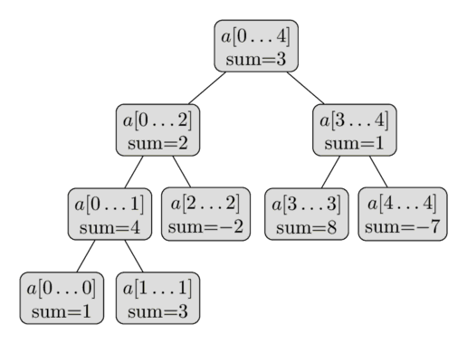
From this short description of the data structure, we can already conclude that a Segment Tree only requires a linear number of vertices. The first level of the tree contains a single node (the root), the second level will contain two vertices, in the third it will contain four vertices, until the number of vertices reaches $n$. Thus the number of vertices in the worst case can be estimated by the sum $1 + 2 + 4 + \dots + 2^{\lceil\log_2 n\rceil} \lt 2^{\lceil\log_2 n\rceil + 1} \lt 4n$.
It is worth noting that whenever $n$ is not a power of two, not all levels of the Segment Tree will be completely filled. We can see that behavior in the image. For now we can forget about this fact, but it will become important later during the implementation.
The height of the Segment Tree is $O(\log n)$, because when going down from the root to the leaves the size of the segments decreases approximately by half.
Construction
Before constructing the segment tree, we need to decide:
- the value that gets stored at each node of the segment tree. For example, in a sum segment tree, a node would store the sum of the elements in its range $[l, r]$.
- the merge operation that merges two siblings in a segment tree. For example, in a sum segment tree, the two nodes corresponding to the ranges $a[l_1 \dots r_1]$ and $a[l_2 \dots r_2]$ would be merged into a node corresponding to the range $a[l_1 \dots r_2]$ by adding the values of the two nodes.
Note that a vertex is a "leaf vertex", if its corresponding segment covers only one value in the original array. It is present at the lowermost level of a segment tree. Its value would be equal to the (corresponding) element $a[i]$.
Now, for construction of the segment tree, we start at the bottom level (the leaf vertices) and assign them their respective values. On the basis of these values, we can compute the values of the previous level, using the merge function.
And on the basis of those, we can compute the values of the previous, and repeat the procedure until we reach the root vertex.
It is convenient to describe this operation recursively in the other direction, i.e., from the root vertex to the leaf vertices. The construction procedure, if called on a non-leaf vertex, does the following:
- recursively construct the values of the two child vertices
- merge the computed values of these children.
We start the construction at the root vertex, and hence, we are able to compute the entire segment tree.
The time complexity of this construction is $O(n)$, assuming that the merge operation is constant time (the merge operation gets called $n$ times, which is equal to the number of internal nodes in the segment tree).
Sum queries
For now we are going to answer sum queries. As an input we receive two integers $l$ and $r$, and we have to compute the sum of the segment $a[l \dots r]$ in $O(\log n)$ time.
To do this, we will traverse the Segment Tree and use the precomputed sums of the segments. Let's assume that we are currently at the vertex that covers the segment $a[tl \dots tr]$. There are three possible cases.
The easiest case is when the segment $a[l \dots r]$ is equal to the corresponding segment of the current vertex (i.e. $a[l \dots r] = a[tl \dots tr]$), then we are finished and can return the precomputed sum that is stored in the vertex.
Alternatively the segment of the query can fall completely into the domain of either the left or the right child. Recall that the left child covers the segment $a[tl \dots tm]$ and the right vertex covers the segment $a[tm + 1 \dots tr]$ with $tm = (tl + tr) / 2$. In this case we can simply go to the child vertex, which corresponding segment covers the query segment, and execute the algorithm described here with that vertex.
And then there is the last case, the query segment intersects with both children. In this case we have no other option as to make two recursive calls, one for each child. First we go to the left child, compute a partial answer for this vertex (i.e. the sum of values of the intersection between the segment of the query and the segment of the left child), then go to the right child, compute the partial answer using that vertex, and then combine the answers by adding them. In other words, since the left child represents the segment $a[tl \dots tm]$ and the right child the segment $a[tm+1 \dots tr]$, we compute the sum query $a[l \dots tm]$ using the left child, and the sum query $a[tm+1 \dots r]$ using the right child.
So processing a sum query is a function that recursively calls itself once with either the left or the right child (without changing the query boundaries), or twice, once for the left and once for the right child (by splitting the query into two subqueries). And the recursion ends, whenever the boundaries of the current query segment coincides with the boundaries of the segment of the current vertex. In that case the answer will be the precomputed value of the sum of this segment, which is stored in the tree.
In other words, the calculation of the query is a traversal of the tree, which spreads through all necessary branches of the tree, and uses the precomputed sum values of the segments in the tree.
Obviously we will start the traversal from the root vertex of the Segment Tree.
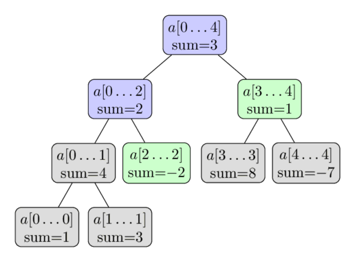
The procedure is illustrated in the following image. Again the array $a = [1, 3, -2, 8, -7]$ is used, and here we want to compute the sum $\sum_{i=2}^4 a[i]$. The colored vertices will be visited, and we will use the precomputed values of the green vertices. This gives us the result $-2 + 1 = -1$.
Why is the complexity of this algorithm $O(\log n)$? To show this complexity we look at each level of the tree. It turns out, that for each level we only visit not more than four vertices. And since the height of the tree is $O(\log n)$, we receive the desired running time.
We can show that this proposition (at most four vertices each level) is true by induction. At the first level, we only visit one vertex, the root vertex, so here we visit less than four vertices. Now let's look at an arbitrary level. By induction hypothesis, we visit at most four vertices. If we only visit at most two vertices, the next level has at most four vertices. That is trivial, because each vertex can only cause at most two recursive calls. So let's assume that we visit three or four vertices in the current level. From those vertices, we will analyze the vertices in the middle more carefully. Since the sum query asks for the sum of a continuous subarray, we know that segments corresponding to the visited vertices in the middle will be completely covered by the segment of the sum query. Therefore these vertices will not make any recursive calls. So only the most left, and the most right vertex will have the potential to make recursive calls. And those will only create at most four recursive calls, so also the next level will satisfy the assertion. We can say that one branch approaches the left boundary of the query, and the second branch approaches the right one.
Therefore we visit at most $4 \log n$ vertices in total, and that is equal to a running time of $O(\log n)$.
In conclusion the query works by dividing the input segment into several sub-segments for which all the sums are already precomputed and stored in the tree. And if we stop partitioning whenever the query segment coincides with the vertex segment, then we only need $O(\log n)$ such segments, which gives the effectiveness of the Segment Tree.
Update queries
Now we want to modify a specific element in the array, let's say we want to do the assignment $a[i] = x$. And we have to rebuild the Segment Tree, such that it corresponds to the new, modified array.
This query is easier than the sum query. Each level of a Segment Tree forms a partition of the array. Therefore an element $a[i]$ only contributes to one segment from each level. Thus only $O(\log n)$ vertices need to be updated.
It is easy to see, that the update request can be implemented using a recursive function. The function gets passed the current tree vertex, and it recursively calls itself with one of the two child vertices (the one that contains $a[i]$ in its segment), and after that recomputes its sum value, similar how it is done in the build method (that is as the sum of its two children).
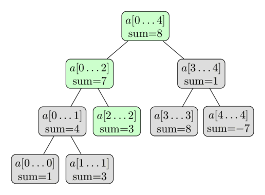
Again here is a visualization using the same array. Here we perform the update $a[2] = 3$. The green vertices are the vertices that we visit and update.
Implementation
The main consideration is how to store the Segment Tree. Of course we can define a $\text{Vertex}$ struct and create objects, that store the boundaries of the segment, its sum and additionally also pointers to its child vertices. However, this requires storing a lot of redundant information in the form of pointers. We will use a simple trick to make this a lot more efficient by using an implicit data structure: Only storing the sums in an array. (A similar method is used for binary heaps). The sum of the root vertex at index 1, the sums of its two child vertices at indices 2 and 3, the sums of the children of those two vertices at indices 4 to 7, and so on. With 1-indexing, conveniently the left child of a vertex at index $i$ is stored at index $2i$, and the right one at index $2i + 1$. Equivalently, the parent of a vertex at index $i$ is stored at $i/2$ (integer division).
This simplifies the implementation a lot. We don't need to store the structure of the tree in memory. It is defined implicitly. We only need one array which contains the sums of all segments.
As noted before, we need to store at most $4n$ vertices. It might be less, but for convenience we always allocate an array of size $4n$. There will be some elements in the sum array, that will not correspond to any vertices in the actual tree, but this doesn't complicate the implementation.
So, we store the Segment Tree simply as an array $t[]$ with a size of four times the input size $n$:
int n, t[4*MAXN];
The procedure for constructing the Segment Tree from a given array $a[]$ looks like this: it is a recursive function with the parameters $a[]$ (the input array), $v$ (the index of the current vertex), and the boundaries $tl$ and $tr$ of the current segment. In the main program this function will be called with the parameters of the root vertex: $v = 1$, $tl = 0$, and $tr = n - 1$.
void build(int a[], int v, int tl, int tr) {
    if (tl == tr) {
        t[v] = a[tl];
    } else {
        int tm = (tl + tr) / 2;
        build(a, v*2, tl, tm);
        build(a, v*2+1, tm+1, tr);
        t[v] = t[v*2] + t[v*2+1];
    }
}
Further the function for answering sum queries is also a recursive function, which receives as parameters information about the current vertex/segment (i.e. the index $v$ and the boundaries $tl$ and $tr$) and also the information about the boundaries of the query, $l$ and $r$. In order to simplify the code, this function always does two recursive calls, even if only one is necessary - in that case the superfluous recursive call will have $l > r$, and this can easily be caught using an additional check at the beginning of the function.
int sum(int v, int tl, int tr, int l, int r) {
    if (l > r)
        return 0;
    if (l == tl && r == tr) {
        return t[v];
    }
    int tm = (tl + tr) / 2;
    return sum(v*2, tl, tm, l, min(r, tm))
           + sum(v*2+1, tm+1, tr, max(l, tm+1), r);
}
Finally the update query. The function will also receive information about the current vertex/segment, and additionally also the parameter of the update query (i.e. the position of the element and its new value).
void update(int v, int tl, int tr, int pos, int new_val) {
    if (tl == tr) {
        t[v] = new_val;
    } else {
        int tm = (tl + tr) / 2;
        if (pos <= tm)
            update(v*2, tl, tm, pos, new_val);
        else
            update(v*2+1, tm+1, tr, pos, new_val);
        t[v] = t[v*2] + t[v*2+1];
    }
}
Memory efficient implementation
Most people use the implementation from the previous section. If you look at the array t you can see that it follows the numbering of the tree nodes in the order of a BFS traversal (level-order traversal).
Using this traversal the children of vertex $v$ are $2v$ and $2v + 1$ respectively.
However if $n$ is not a power of two, this method will skip some indices and leave some parts of the array t unused.
The memory consumption is limited by $4n$, even though a Segment Tree of an array of $n$ elements requires only $2n - 1$ vertices.
However it can be reduced. We renumber the vertices of the tree in the order of an Euler tour traversal (pre-order traversal), and we write all these vertices next to each other.
Let's look at a vertex at index $v$, and let it be responsible for the segment $[l, r]$, and let $mid = \dfrac{l + r}{2}$. It is obvious that the left child will have the index $v + 1$. The left child is responsible for the segment $[l, mid]$, i.e. in total there will be $2 * (mid - l + 1) - 1$ vertices in the left child's subtree. Thus we can compute the index of the right child of $v$. The index will be $v + 2 * (mid - l + 1)$. By this numbering we achieve a reduction of the necessary memory to $2n$.
Advanced versions of Segment Trees
A Segment Tree is a very flexible data structure, and allows variations and extensions in many different directions. Let's try to categorize them below.
More complex queries
It can be quite easy to change the Segment Tree in a direction, such that it computes different queries (e.g. computing the minimum / maximum instead of the sum), but it also can be very nontrivial.
Finding the maximum
Let us slightly change the condition of the problem described above: instead of querying the sum, we will now make maximum queries.
The tree will have exactly the same structure as the tree described above. We only need to change the way $t[v]$ is computed in the $\text{build}$ and $\text{update}$ functions. $t[v]$ will now store the maximum of the corresponding segment. And we also need to change the calculation of the returned value of the $\text{sum}$ function (replacing the summation by the maximum).
Of course this problem can be easily changed into computing the minimum instead of the maximum.
Instead of showing an implementation to this problem, the implementation will be given to a more complex version of this problem in the next section.
Finding the maximum and the number of times it appears
This task is very similar to the previous one. In addition of finding the maximum, we also have to find the number of occurrences of the maximum.
To solve this problem, we store a pair of numbers at each vertex in the tree: In addition to the maximum we also store the number of occurrences of it in the corresponding segment. Determining the correct pair to store at $t[v]$ can still be done in constant time using the information of the pairs stored at the child vertices. Combining two such pairs should be done in a separate function, since this will be an operation that we will do while building the tree, while answering maximum queries and while performing modifications.
pair<int, int> t[4*MAXN];

pair<int, int> combine(pair<int, int> a, pair<int, int> b) {
    if (a.first > b.first)
        return a;
    if (b.first > a.first)
        return b;
    return make_pair(a.first, a.second + b.second);
}

void build(int a[], int v, int tl, int tr) {
    if (tl == tr) {
        t[v] = make_pair(a[tl], 1);
    } else {
        int tm = (tl + tr) / 2;
        build(a, v*2, tl, tm);
        build(a, v*2+1, tm+1, tr);
        t[v] = combine(t[v*2], t[v*2+1]);
    }
}

pair<int, int> get_max(int v, int tl, int tr, int l, int r) {
    if (l > r)
        return make_pair(-INF, 0);
    if (l == tl && r == tr)
        return t[v];
    int tm = (tl + tr) / 2;
    return combine(get_max(v*2, tl, tm, l, min(r, tm)),
                   get_max(v*2+1, tm+1, tr, max(l, tm+1), r));
}

void update(int v, int tl, int tr, int pos, int new_val) {
    if (tl == tr) {
        t[v] = make_pair(new_val, 1);
    } else {
        int tm = (tl + tr) / 2;
        if (pos <= tm)
            update(v*2, tl, tm, pos, new_val);
        else
            update(v*2+1, tm+1, tr, pos, new_val);
        t[v] = combine(t[v*2], t[v*2+1]);
    }
}
Compute the greatest common divisor / least common multiple
In this problem we want to compute the GCD / LCM of all numbers of given ranges of the array.
This interesting variation of the Segment Tree can be solved in exactly the same way as the Segment Trees we derived for sum / minimum / maximum queries: it is enough to store the GCD / LCM of the corresponding vertex in each vertex of the tree. Combining two vertices can be done by computing the GCD / LCM of both vertices.
Counting the number of zeros, searching for the $k$-th zero
In this problem we want to find the number of zeros in a given range, and additionally find the index of the $k$-th zero using a second function.
Again we have to change the store values of the tree a bit: This time we will store the number of zeros in each segment in $t[]$. It is pretty clear, how to implement the $\text{build}$, $\text{update}$ and $\text{count_zero}$ functions, we can simply use the ideas from the sum query problem. Thus we solved the first part of the problem.
Now we learn how to solve the problem of finding the $k$-th zero in the array $a[]$. To do this task, we will descend the Segment Tree, starting at the root vertex, and moving each time to either the left or the right child, depending on which segment contains the $k$-th zero. In order to decide to which child we need to go, it is enough to look at the number of zeros appearing in the segment corresponding to the left vertex. If this precomputed count is greater or equal to $k$, it is necessary to descend to the left child, and otherwise descent to the right child. Notice, if we chose the right child, we have to subtract the number of zeros of the left child from $k$.
In the implementation we can handle the special case, $a[]$ containing less than $k$ zeros, by returning -1.
int find_kth(int v, int tl, int tr, int k) {
    if (k > t[v])
        return -1;
    if (tl == tr)
        return tl;
    int tm = (tl + tr) / 2;
    if (t[v*2] >= k)
        return find_kth(v*2, tl, tm, k);
    else
        return find_kth(v*2+1, tm+1, tr, k - t[v*2]);
}
Searching for an array prefix with a given amount
The task is as follows: for a given value $x$ we have to quickly find smallest index $i$ such that the sum of the first $i$ elements of the array $a[]$ is greater or equal to $x$ (assuming that the array $a[]$ only contains non-negative values).
This task can be solved using binary search, computing the sum of the prefixes with the Segment Tree. However this will lead to a $O(\log^2 n)$ solution.
Instead we can use the same idea as in the previous section, and find the position by descending the tree: by moving each time to the left or the right, depending on the sum of the left child. Thus finding the answer in $O(\log n)$ time.
Searching for the first element greater than a given amount
The task is as follows: for a given value $x$ and a range $a[l \dots r]$ find the smallest $i$ in the range $a[l \dots r]$, such that $a[i]$ is greater than $x$.
This task can be solved using binary search over max prefix queries with the Segment Tree. However, this will lead to a $O(\log^2 n)$ solution.
Instead, we can use the same idea as in the previous sections, and find the position by descending the tree: by moving each time to the left or the right, depending on the maximum value of the left child. Thus finding the answer in $O(\log n)$ time.
int get_first(int v, int tl, int tr, int l, int r, int x) {
    if(tl > r || tr < l) return -1;
    if(t[v] <= x) return -1;

    if (tl== tr) return tl;

    int tm = tl + (tr-tl)/2;
    int left = get_first(2*v, tl, tm, l, r, x);
    if(left != -1) return left;
    return get_first(2*v+1, tm+1, tr, l ,r, x);
}
Finding subsegments with the maximal sum
Here again we receive a range $a[l \dots r]$ for each query, this time we have to find a subsegment $a[l^\prime \dots r^\prime]$ such that $l \le l^\prime$ and $r^\prime \le r$ and the sum of the elements of this segment is maximal. As before we also want to be able to modify individual elements of the array. The elements of the array can be negative, and the optimal subsegment can be empty (e.g. if all elements are negative).
This problem is a non-trivial usage of a Segment Tree. This time we will store four values for each vertex: the sum of the segment, the maximum prefix sum, the maximum suffix sum, and the sum of the maximal subsegment in it. In other words for each segment of the Segment Tree the answer is already precomputed as well as the answers for segments touching the left and the right boundaries of the segment.
How to build a tree with such data? Again we compute it in a recursive fashion: we first compute all four values for the left and the right child, and then combine those to archive the four values for the current vertex. Note the answer for the current vertex is either:
- the answer of the left child, which means that the optimal subsegment is entirely placed in the segment of the left child
- the answer of the right child, which means that the optimal subsegment is entirely placed in the segment of the right child
- the sum of the maximum suffix sum of the left child and the maximum prefix sum of the right child, which means that the optimal subsegment intersects with both children.
Hence the answer to the current vertex is the maximum of these three values. Computing the maximum prefix / suffix sum is even easier. Here is the implementation of the $\text{combine}$ function, which receives only data from the left and right child, and returns the data of the current vertex.
struct data {
    int sum, pref, suff, ans;
};

data combine(data l, data r) {
    data res;
    res.sum = l.sum + r.sum;
    res.pref = max(l.pref, l.sum + r.pref);
    res.suff = max(r.suff, r.sum + l.suff);
    res.ans = max(max(l.ans, r.ans), l.suff + r.pref);
    return res;
}
Using the $\text{combine}$ function it is easy to build the Segment Tree. We can implement it in exactly the same way as in the previous implementations. To initialize the leaf vertices, we additionally create the auxiliary function $\text{make_data}$, which will return a $\text{data}$ object holding the information of a single value.
data make_data(int val) {
    data res;
    res.sum = val;
    res.pref = res.suff = res.ans = max(0, val);
    return res;
}

void build(int a[], int v, int tl, int tr) {
    if (tl == tr) {
        t[v] = make_data(a[tl]);
    } else {
        int tm = (tl + tr) / 2;
        build(a, v*2, tl, tm);
        build(a, v*2+1, tm+1, tr);
        t[v] = combine(t[v*2], t[v*2+1]);
    }
}

void update(int v, int tl, int tr, int pos, int new_val) {
    if (tl == tr) {
        t[v] = make_data(new_val);
    } else {
        int tm = (tl + tr) / 2;
        if (pos <= tm)
            update(v*2, tl, tm, pos, new_val);
        else
            update(v*2+1, tm+1, tr, pos, new_val);
        t[v] = combine(t[v*2], t[v*2+1]);
    }
}
It only remains, how to compute the answer to a query. To answer it, we go down the tree as before, breaking the query into several subsegments that coincide with the segments of the Segment Tree, and combine the answers in them into a single answer for the query. Then it should be clear, that the work is exactly the same as in the simple Segment Tree, but instead of summing / minimizing / maximizing the values, we use the $\text{combine}$ function.
data query(int v, int tl, int tr, int l, int r) {
    if (l > r)
        return make_data(0);
    if (l == tl && r == tr)
        return t[v];
    int tm = (tl + tr) / 2;
    return combine(query(v*2, tl, tm, l, min(r, tm)),
                   query(v*2+1, tm+1, tr, max(l, tm+1), r));
}
Saving the entire subarrays in each vertex
This is a separate subsection that stands apart from the others, because at each vertex of the Segment Tree we don't store information about the corresponding segment in compressed form (sum, minimum, maximum, ...), but store all elements of the segment. Thus the root of the Segment Tree will store all elements of the array, the left child vertex will store the first half of the array, the right vertex the second half, and so on.
In its simplest application of this technique we store the elements in sorted order. In more complex versions the elements are not stored in lists, but more advanced data structures (sets, maps, ...). But all these methods have the common factor, that each vertex requires linear memory (i.e. proportional to the length of the corresponding segment).
The first natural question, when considering these Segment Trees, is about memory consumption. Intuitively this might look like $O(n^2)$ memory, but it turns out that the complete tree will only need $O(n \log n)$ memory. Why is this so? Quite simply, because each element of the array falls into $O(\log n)$ segments (remember the height of the tree is $O(\log n)$).
So in spite of the apparent extravagance of such a Segment Tree, it consumes only slightly more memory than the usual Segment Tree.
Several typical applications of this data structure are described below. It is worth noting the similarity of these Segment Trees with 2D data structures (in fact this is a 2D data structure, but with rather limited capabilities).
Find the smallest number greater or equal to a specified number. No modification queries.
We want to answer queries of the following form: for three given numbers $(l, r, x)$ we have to find the minimal number in the segment $a[l \dots r]$ which is greater than or equal to $x$.
We construct a Segment Tree. In each vertex we store a sorted list of all numbers occurring in the corresponding segment, like described above. How to build such a Segment Tree as effectively as possible? As always we approach this problem recursively: let the lists of the left and right children already be constructed, and we want to build the list for the current vertex. From this view the operation is now trivial and can be accomplished in linear time: We only need to combine the two sorted lists into one, which can be done by iterating over them using two pointers. The C++ STL already has an implementation of this algorithm.
Because this structure of the Segment Tree and the similarities to the merge sort algorithm, the data structure is also often called "Merge Sort Tree".
vector<int> t[4*MAXN];

void build(int a[], int v, int tl, int tr) {
    if (tl == tr) {
        t[v] = vector<int>(1, a[tl]);
    } else {
        int tm = (tl + tr) / 2;
        build(a, v*2, tl, tm);
        build(a, v*2+1, tm+1, tr);
        merge(t[v*2].begin(), t[v*2].end(), t[v*2+1].begin(), t[v*2+1].end(),
              back_inserter(t[v]));
    }
}
We already know that the Segment Tree constructed in this way will require $O(n \log n)$ memory. And thanks to this implementation its construction also takes $O(n \log n)$ time, after all each list is constructed in linear time in respect to its size.
Now consider the answer to the query. We will go down the tree, like in the regular Segment Tree, breaking our segment $a[l \dots r]$ into several subsegments (into at most $O(\log n)$ pieces). It is clear that the answer of the whole answer is the minimum of each of the subqueries. So now we only need to understand, how to respond to a query on one such subsegment that corresponds with some vertex of the tree.
We are at some vertex of the Segment Tree and we want to compute the answer to the query, i.e. find the minimum number greater that or equal to a given number $x$. Since the vertex contains the list of elements in sorted order, we can simply perform a binary search on this list and return the first number, greater than or equal to $x$.
Thus the answer to the query in one segment of the tree takes $O(\log n)$ time, and the entire query is processed in $O(\log^2 n)$.
int query(int v, int tl, int tr, int l, int r, int x) {
    if (l > r)
        return INF;
    if (l == tl && r == tr) {
        vector<int>::iterator pos = lower_bound(t[v].begin(), t[v].end(), x);
        if (pos != t[v].end())
            return *pos;
        return INF;
    }
    int tm = (tl + tr) / 2;
    return min(query(v*2, tl, tm, l, min(r, tm), x),
               query(v*2+1, tm+1, tr, max(l, tm+1), r, x));
}
The constant $\text{INF}$ is equal to some large number that is bigger than all numbers in the array. Its usage means, that there is no number greater than or equal to $x$ in the segment. It has the meaning of "there is no answer in the given interval".
Find the smallest number greater or equal to a specified number. With modification queries.
This task is similar to the previous. The last approach has a disadvantage, it was not possible to modify the array between answering queries. Now we want to do exactly this: a modification query will do the assignment $a[i] = y$.
The solution is similar to the solution of the previous problem, but instead of lists at each vertex of the Segment Tree, we will store a balanced list that allows you to quickly search for numbers, delete numbers, and insert new numbers. Since the array can contain a number repeated, the optimal choice is the data structure $\text{multiset}$.
The construction of such a Segment Tree is done in pretty much the same way as in the previous problem, only now we need to combine $\text{multiset}$s and not sorted lists. This leads to a construction time of $O(n \log^2 n)$ (in general merging two red-black trees can be done in linear time, but the C++ STL doesn't guarantee this time complexity).
The $\text{query}$ function is also almost equivalent, only now the $\text{lower_bound}$ function of the $\text{multiset}$ function should be called instead ($\text{std::lower_bound}$ only works in $O(\log n)$ time if used with random-access iterators).
Finally the modification request. To process it, we must go down the tree, and modify all $\text{multiset}$ from the corresponding segments that contain the affected element. We simply delete the old value of this element (but only one occurrence), and insert the new value.
void update(int v, int tl, int tr, int pos, int new_val) {
    t[v].erase(t[v].find(a[pos]));
    t[v].insert(new_val);
    if (tl != tr) {
        int tm = (tl + tr) / 2;
        if (pos <= tm)
            update(v*2, tl, tm, pos, new_val);
        else
            update(v*2+1, tm+1, tr, pos, new_val);
    } else {
        a[pos] = new_val;
    }
}
Processing of this modification query also takes $O(\log^2 n)$ time.
Find the smallest number greater or equal to a specified number. Acceleration with "fractional cascading".
We have the same problem statement, we want to find the minimal number greater than or equal to $x$ in a segment, but this time in $O(\log n)$ time. We will improve the time complexity using the technique "fractional cascading".
Fractional cascading is a simple technique that allows you to improve the running time of multiple binary searches, which are conducted at the same time. Our previous approach to the search query was, that we divide the task into several subtasks, each of which is solved with a binary search. Fractional cascading allows you to replace all of these binary searches with a single one.
The simplest and most obvious example of fractional cascading is the following problem: there are $k$ sorted lists of numbers, and we must find in each list the first number greater than or equal to the given number.
Instead of performing a binary search for each list, we could merge all lists into one big sorted list. Additionally for each element $y$ we store a list of results of searching for $y$ in each of the $k$ lists. Therefore if we want to find the smallest number greater than or equal to $x$, we just need to perform one single binary search, and from the list of indices we can determine the smallest number in each list. This approach however requires $O(n \cdot k)$ ($n$ is the length of the combined lists), which can be quite inefficient.
Fractional cascading reduces this memory complexity to $O(n)$ memory, by creating from the $k$ input lists $k$ new lists, in which each list contains the corresponding list and additionally also every second element of the following new list. Using this structure it is only necessary to store two indices, the index of the element in the original list, and the index of the element in the following new list. So this approach only uses $O(n)$ memory, and still can answer the queries using a single binary search.
But for our application we do not need the full power of fractional cascading. In our Segment Tree a vertex will contain the sorted list of all elements that occur in either the left or the right subtrees (like in the Merge Sort Tree). Additionally to this sorted list, we store two positions for each element. For an element $y$ we store the smallest index $i$, such that the $i$th element in the sorted list of the left child is greater or equal to $y$. And we store the smallest index $j$, such that the $j$th element in the sorted list of the right child is greater or equal to $y$. These values can be computed in parallel to the merging step when we build the tree.
How does this speed up the queries?
Remember, in the normal solution we did a binary search in every node. But with this modification, we can avoid all except one.
To answer a query, we simply do a binary search in the root node. This gives us the smallest element $y \ge x$ in the complete array, but it also gives us two positions. The index of the smallest element greater or equal $x$ in the left subtree, and the index of the smallest element $y$ in the right subtree. Notice that $\ge y$ is the same as $\ge x$, since our array doesn't contain any elements between $x$ and $y$. In the normal Merge Sort Tree solution we would compute these indices via binary search, but with the help of the precomputed values we can just look them up in $O(1)$. And we can repeat that until we visited all nodes that cover our query interval.
To summarize, as usual we touch $O(\log n)$ nodes during a query. In the root node we do a binary search, and in all other nodes we only do constant work. This means the complexity for answering a query is $O(\log n)$.
But notice, that this uses three times more memory than a normal Merge Sort Tree, which already uses a lot of memory ($O(n \log n)$).
It is straightforward to apply this technique to a problem, that doesn't require any modification queries. The two positions are just integers and can easily be computed by counting when merging the two sorted sequences.
It is still possible to also allow modification queries, but that complicates the entire code.
Instead of integers, you need to store the sorted array as multiset, and instead of indices you need to store iterators.
And you need to work very carefully, so that you increment or decrement the correct iterators during a modification query.
Other possible variations
This technique implies a whole new class of possible applications. Instead of storing a $\text{vector}$ or a $\text{multiset}$ in each vertex, other data structures can be used: other Segment Trees (somewhat discussed in Generalization to higher dimensions), Fenwick Trees, Cartesian trees, etc.
Range updates (Lazy Propagation)
All problems in the above sections discussed modification queries that only affected a single element of the array each. However the Segment Tree allows applying modification queries to an entire segment of contiguous elements, and perform the query in the same time $O(\log n)$.
Addition on segments
We begin by considering problems of the simplest form: the modification query should add a number $x$ to all numbers in the segment $a[l \dots r]$. The second query, that we are supposed to answer, asked simply for the value of $a[i]$.
To make the addition query efficient, we store at each vertex in the Segment Tree how many we should add to all numbers in the corresponding segment. For example, if the query "add 3 to the whole array $a[0 \dots n-1]$" comes, then we place the number 3 in the root of the tree. In general we have to place this number to multiple segments, which form a partition of the query segment. Thus we don't have to change all $O(n)$ values, but only $O(\log n)$ many.
If now there comes a query that asks the current value of a particular array entry, it is enough to go down the tree and add up all values found along the way.
void build(int a[], int v, int tl, int tr) {
    if (tl == tr) {
        t[v] = a[tl];
    } else {
        int tm = (tl + tr) / 2;
        build(a, v*2, tl, tm);
        build(a, v*2+1, tm+1, tr);
        t[v] = 0;
    }
}

void update(int v, int tl, int tr, int l, int r, int add) {
    if (l > r)
        return;
    if (l == tl && r == tr) {
        t[v] += add;
    } else {
        int tm = (tl + tr) / 2;
        update(v*2, tl, tm, l, min(r, tm), add);
        update(v*2+1, tm+1, tr, max(l, tm+1), r, add);
    }
}

int get(int v, int tl, int tr, int pos) {
    if (tl == tr)
        return t[v];
    int tm = (tl + tr) / 2;
    if (pos <= tm)
        return t[v] + get(v*2, tl, tm, pos);
    else
        return t[v] + get(v*2+1, tm+1, tr, pos);
}
Assignment on segments
Suppose now that the modification query asks to assign each element of a certain segment $a[l \dots r]$ to some value $p$. As a second query we will again consider reading the value of the array $a[i]$.
To perform this modification query on a whole segment, you have to store at each vertex of the Segment Tree whether the corresponding segment is covered entirely with the same value or not. This allows us to make a "lazy" update: instead of changing all segments in the tree that cover the query segment, we only change some, and leave others unchanged. A marked vertex will mean, that every element of the corresponding segment is assigned to that value, and actually also the complete subtree should only contain this value. In a sense we are lazy and delay writing the new value to all those vertices. We can do this tedious task later, if this is necessary.
So after the modification query is executed, some parts of the tree become irrelevant - some modifications remain unfulfilled in it.
For example if a modification query "assign a number to the whole array $a[0 \dots n-1]$" gets executed, in the Segment Tree only a single change is made - the number is placed in the root of the tree and this vertex gets marked. The remaining segments remain unchanged, although in fact the number should be placed in the whole tree.
Suppose now that the second modification query says, that the first half of the array $a[0 \dots n/2]$ should be assigned with some other number. To process this query we must assign each element in the whole left child of the root vertex with that number. But before we do this, we must first sort out the root vertex first. The subtlety here is that the right half of the array should still be assigned to the value of the first query, and at the moment there is no information for the right half stored.
The way to solve this is to push the information of the root to its children, i.e. if the root of the tree was assigned with any number, then we assign the left and the right child vertices with this number and remove the mark of the root. After that, we can assign the left child with the new value, without losing any necessary information.
Summarizing we get: for any queries (a modification or reading query) during the descent along the tree we should always push information from the current vertex into both of its children. We can understand this in such a way, that when we descent the tree we apply delayed modifications, but exactly as much as necessary (so not to degrade the complexity of $O(\log n)$).
For the implementation we need to make a $\text{push}$ function, which will receive the current vertex, and it will push the information for its vertex to both its children. We will call this function at the beginning of the query functions (but we will not call it from the leaves, because there is no need to push information from them any further).
void push(int v) {
    if (marked[v]) {
        t[v*2] = t[v*2+1] = t[v];
        marked[v*2] = marked[v*2+1] = true;
        marked[v] = false;
    }
}

void update(int v, int tl, int tr, int l, int r, int new_val) {
    if (l > r)
        return;
    if (l == tl && tr == r) {
        t[v] = new_val;
        marked[v] = true;
    } else {
        push(v);
        int tm = (tl + tr) / 2;
        update(v*2, tl, tm, l, min(r, tm), new_val);
        update(v*2+1, tm+1, tr, max(l, tm+1), r, new_val);
    }
}

int get(int v, int tl, int tr, int pos) {
    if (tl == tr) {
        return t[v];
    }
    push(v);
    int tm = (tl + tr) / 2;
    if (pos <= tm)
        return get(v*2, tl, tm, pos);
    else
        return get(v*2+1, tm+1, tr, pos);
}
Notice: the function $\text{get}$ can also be implemented in a different way: do not make delayed updates, but immediately return the value $t[v]$ if $marked[v]$ is true.
Adding on segments, querying for maximum
Now the modification query is to add a number to all elements in a range, and the reading query is to find the maximum in a range.
So for each vertex of the Segment Tree we have to store the maximum of the corresponding subsegment. The interesting part is how to recompute these values during a modification request.
For this purpose we store an additional value for each vertex. In this value we store the addends we haven't propagated to the child vertices. Before traversing to a child vertex, we call $\text{push}$ and propagate the value to both children. We have to do this in both the $\text{update}$ function and the $\text{query}$ function.
void build(int a[], int v, int tl, int tr) {
    if (tl == tr) {
        t[v] = a[tl];
    } else {
        int tm = (tl + tr) / 2;
        build(a, v*2, tl, tm);
        build(a, v*2+1, tm+1, tr);
        t[v] = max(t[v*2], t[v*2 + 1]);
    }
}

void push(int v) {
    t[v*2] += lazy[v];
    lazy[v*2] += lazy[v];
    t[v*2+1] += lazy[v];
    lazy[v*2+1] += lazy[v];
    lazy[v] = 0;
}

void update(int v, int tl, int tr, int l, int r, int addend) {
    if (l > r)
        return;
    if (l == tl && tr == r) {
        t[v] += addend;
        lazy[v] += addend;
    } else {
        push(v);
        int tm = (tl + tr) / 2;
        update(v*2, tl, tm, l, min(r, tm), addend);
        update(v*2+1, tm+1, tr, max(l, tm+1), r, addend);
        t[v] = max(t[v*2], t[v*2+1]);
    }
}

int query(int v, int tl, int tr, int l, int r) {
    if (l > r)
        return -INF;
    if (l == tl && tr == r)
        return t[v];
    push(v);
    int tm = (tl + tr) / 2;
    return max(query(v*2, tl, tm, l, min(r, tm)),
               query(v*2+1, tm+1, tr, max(l, tm+1), r));
}
Generalization to higher dimensions
A Segment Tree can be generalized quite natural to higher dimensions. If in the one-dimensional case we split the indices of the array into segments, then in the two-dimensional we make an ordinary Segment Tree with respect to the first indices, and for each segment we build an ordinary Segment Tree with respect to the second indices.
Simple 2D Segment Tree
A matrix $a[0 \dots n-1, 0 \dots m-1]$ is given, and we have to find the sum (or minimum/maximum) on some submatrix $a[x_1 \dots x_2, y_1 \dots y_2]$, as well as perform modifications of individual matrix elements (i.e. queries of the form $a[x][y] = p$).
So we build a 2D Segment Tree: first the Segment Tree using the first coordinate ($x$), then the second ($y$).
To make the construction process more understandable, you can forget for a while that the matrix is two-dimensional, and only leave the first coordinate. We will construct an ordinary one-dimensional Segment Tree using only the first coordinate. But instead of storing a number in a segment, we store an entire Segment Tree: i.e. at this moment we remember that we also have a second coordinate; but because at this moment the first coordinate is already fixed to some interval $[l \dots r]$, we actually work with such a strip $a[l \dots r, 0 \dots m-1]$ and for it we build a Segment Tree.
Here is the implementation of the construction of a 2D Segment Tree. It actually represents two separate blocks: the construction of a Segment Tree along the $x$ coordinate ($\text{build}_x$), and the $y$ coordinate ($\text{build}_y$). For the leaf nodes in $\text{build}_y$ we have to separate two cases: when the current segment of the first coordinate $[tlx \dots trx]$ has length 1, and when it has a length greater than one. In the first case, we just take the corresponding value from the matrix, and in the second case we can combine the values of two Segment Trees from the left and the right son in the coordinate $x$.
void build_y(int vx, int lx, int rx, int vy, int ly, int ry) {
    if (ly == ry) {
        if (lx == rx)
            t[vx][vy] = a[lx][ly];
        else
            t[vx][vy] = t[vx*2][vy] + t[vx*2+1][vy];
    } else {
        int my = (ly + ry) / 2;
        build_y(vx, lx, rx, vy*2, ly, my);
        build_y(vx, lx, rx, vy*2+1, my+1, ry);
        t[vx][vy] = t[vx][vy*2] + t[vx][vy*2+1];
    }
}

void build_x(int vx, int lx, int rx) {
    if (lx != rx) {
        int mx = (lx + rx) / 2;
        build_x(vx*2, lx, mx);
        build_x(vx*2+1, mx+1, rx);
    }
    build_y(vx, lx, rx, 1, 0, m-1);
}
Such a Segment Tree still uses a linear amount of memory, but with a larger constant: $16 n m$. It is clear that the described procedure $\text{build}_x$ also works in linear time.
Now we turn to processing of queries. We will answer to the two-dimensional query using the same principle: first break the query on the first coordinate, and then for every reached vertex, we call the corresponding Segment Tree of the second coordinate.
int sum_y(int vx, int vy, int tly, int try_, int ly, int ry) {
    if (ly > ry)
        return 0;
    if (ly == tly && try_ == ry)
        return t[vx][vy];
    int tmy = (tly + try_) / 2;
    return sum_y(vx, vy*2, tly, tmy, ly, min(ry, tmy))
         + sum_y(vx, vy*2+1, tmy+1, try_, max(ly, tmy+1), ry);
}

int sum_x(int vx, int tlx, int trx, int lx, int rx, int ly, int ry) {
    if (lx > rx)
        return 0;
    if (lx == tlx && trx == rx)
        return sum_y(vx, 1, 0, m-1, ly, ry);
    int tmx = (tlx + trx) / 2;
    return sum_x(vx*2, tlx, tmx, lx, min(rx, tmx), ly, ry)
         + sum_x(vx*2+1, tmx+1, trx, max(lx, tmx+1), rx, ly, ry);
}
This function works in $O(\log n \log m)$ time, since it first descends the tree in the first coordinate, and for each traversed vertex in the tree it makes a query in the corresponding Segment Tree along the second coordinate.
Finally we consider the modification query. We want to learn how to modify the Segment Tree in accordance with the change in the value of some element $a[x][y] = p$. It is clear, that the changes will occur only in those vertices of the first Segment Tree that cover the coordinate $x$ (and such will be $O(\log n)$), and for Segment Trees corresponding to them the changes will only occurs at those vertices that covers the coordinate $y$ (and such will be $O(\log m)$). Therefore the implementation will be not very different form the one-dimensional case, only now we first descend the first coordinate, and then the second.
void update_y(int vx, int lx, int rx, int vy, int ly, int ry, int x, int y, int new_val) {
    if (ly == ry) {
        if (lx == rx)
            t[vx][vy] = new_val;
        else
            t[vx][vy] = t[vx*2][vy] + t[vx*2+1][vy];
    } else {
        int my = (ly + ry) / 2;
        if (y <= my)
            update_y(vx, lx, rx, vy*2, ly, my, x, y, new_val);
        else
            update_y(vx, lx, rx, vy*2+1, my+1, ry, x, y, new_val);
        t[vx][vy] = t[vx][vy*2] + t[vx][vy*2+1];
    }
}

void update_x(int vx, int lx, int rx, int x, int y, int new_val) {
    if (lx != rx) {
        int mx = (lx + rx) / 2;
        if (x <= mx)
            update_x(vx*2, lx, mx, x, y, new_val);
        else
            update_x(vx*2+1, mx+1, rx, x, y, new_val);
    }
    update_y(vx, lx, rx, 1, 0, m-1, x, y, new_val);
}
Compression of 2D Segment Tree
Let the problem be the following: there are $n$ points on the plane given by their coordinates $(x_i, y_i)$ and queries of the form "count the number of points lying in the rectangle $((x_1, y_1), (x_2, y_2))$". It is clear that in the case of such a problem it becomes unreasonably wasteful to construct a two-dimensional Segment Tree with $O(n^2)$ elements. Most on this memory will be wasted, since each single point can only get into $O(\log n)$ segments of the tree along the first coordinate, and therefore the total "useful" size of all tree segments on the second coordinate is $O(n \log n)$.
So we proceed as follows: at each vertex of the Segment Tree with respect to the first coordinate we store a Segment Tree constructed only by those second coordinates that occur in the current segment of the first coordinates. In other words, when constructing a Segment Tree inside some vertex with index $vx$ and the boundaries $tlx$ and $trx$, we only consider those points that fall into this interval $x \in [tlx, trx]$, and build a Segment Tree just using them.
Thus we will achieve that each Segment Tree on the second coordinate will occupy exactly as much memory as it should. As a result, the total amount of memory will decrease to $O(n \log n)$. We still can answer the queries in $O(\log^2 n)$ time, we just have to make a binary search on the second coordinate, but this will not worsen the complexity.
But modification queries will be impossible with this structure: in fact if a new point appears, we have to add a new element in the middle of some Segment Tree along the second coordinate, which cannot be effectively done.
In conclusion we note that the two-dimensional Segment Tree contracted in the described way becomes practically equivalent to the modification of the one-dimensional Segment Tree (see Saving the entire subarrays in each vertex). In particular the two-dimensional Segment Tree is just a special case of storing a subarray in each vertex of the tree. It follows, that if you gave to abandon a two-dimensional Segment Tree due to the impossibility of executing a query, it makes sense to try to replace the nested Segment Tree with some more powerful data structure, for example a Cartesian tree.
Preserving the history of its values (Persistent Segment Tree)
A persistent data structure is a data structure that remembers it previous state for each modification. This allows to access any version of this data structure that interest us and execute a query on it.
Segment Tree is a data structure that can be turned into a persistent data structure efficiently (both in time and memory consumption). We want to avoid copying the complete tree before each modification, and we don't want to loose the $O(\log n)$ time behavior for answering range queries.
In fact, any change request in the Segment Tree leads to a change in the data of only $O(\log n)$ vertices along the path starting from the root. So if we store the Segment Tree using pointers (i.e. a vertex stores pointers to the left and the right child vertices), then when performing the modification query, we simply need to create new vertices instead of changing the available vertices. Vertices that are not affected by the modification query can still be used by pointing the pointers to the old vertices. Thus for a modification query $O(\log n)$ new vertices will be created, including a new root vertex of the Segment Tree, and the entire previous version of the tree rooted at the old root vertex will remain unchanged.
Let's give an example implementation for the simplest Segment Tree: when there is only a query asking for sums, and modification queries of single elements.
struct Vertex {
    Vertex *l, *r;
    int sum;

    Vertex(int val) : l(nullptr), r(nullptr), sum(val) {}
    Vertex(Vertex *l, Vertex *r) : l(l), r(r), sum(0) {
        if (l) sum += l->sum;
        if (r) sum += r->sum;
    }
};

Vertex* build(int a[], int tl, int tr) {
    if (tl == tr)
        return new Vertex(a[tl]);
    int tm = (tl + tr) / 2;
    return new Vertex(build(a, tl, tm), build(a, tm+1, tr));
}

int get_sum(Vertex* v, int tl, int tr, int l, int r) {
    if (l > r)
        return 0;
    if (l == tl && tr == r)
        return v->sum;
    int tm = (tl + tr) / 2;
    return get_sum(v->l, tl, tm, l, min(r, tm))
         + get_sum(v->r, tm+1, tr, max(l, tm+1), r);
}

Vertex* update(Vertex* v, int tl, int tr, int pos, int new_val) {
    if (tl == tr)
        return new Vertex(new_val);
    int tm = (tl + tr) / 2;
    if (pos <= tm)
        return new Vertex(update(v->l, tl, tm, pos, new_val), v->r);
    else
        return new Vertex(v->l, update(v->r, tm+1, tr, pos, new_val));
}
For each modification of the Segment Tree we will receive a new root vertex. To quickly jump between two different versions of the Segment Tree, we need to store this roots in an array. To use a specific version of the Segment Tree we simply call the query using the appropriate root vertex.
With the approach described above almost any Segment Tree can be turned into a persistent data structure.
Finding the $k$-th smallest number in a range
This time we have to answer queries of the form "What is the $k$-th smallest element in the range $a[l \dots r]$. This query can be answered using a binary search and a Merge Sort Tree, but the time complexity for a single query would be $O(\log^3 n)$. We will accomplish the same task using a persistent Segment Tree in $O(\log n)$.
First we will discuss a solution for a simpler problem: We will only consider arrays in which the elements are bound by $0 \le a[i] \lt n$. And we only want to find the $k$-th smallest element in some prefix of the array $a$. It will be very easy to extent the developed ideas later for not restricted arrays and not restricted range queries. Note that we will be using 1 based indexing for $a$.
We will use a Segment Tree that counts all appearing numbers, i.e. in the Segment Tree we will store the histogram of the array. So the leaf vertices will store how often the values $0$, $1$, $\dots$, $n-1$ will appear in the array, and the other vertices store how many numbers in some range are in the array. In other words we create a regular Segment Tree with sum queries over the histogram of the array. But instead of creating all $n$ Segment Trees for every possible prefix, we will create one persistent one, that will contain the same information. We will start with an empty Segment Tree (all counts will be $0$) pointed to by $root_0$, and add the elements $a[1]$, $a[2]$, $\dots$, $a[n]$ one after another. For each modification we will receive a new root vertex, let's call $root_i$ the root of the Segment Tree after inserting the first $i$ elements of the array $a$. The Segment Tree rooted at $root_i$ will contain the histogram of the prefix $a[1 \dots i]$. Using this Segment Tree we can find in $O(\log n)$ time the position of the $k$-th element using the same technique discussed in Counting the number of zeros, searching for the $k$-th zero.
Now to the not-restricted version of the problem.
First for the restriction on the queries: Instead of only performing these queries over a prefix of $a$, we want to use any arbitrary segments $a[l \dots r]$. Here we need a Segment Tree that represents the histogram of the elements in the range $a[l \dots r]$. It is easy to see that such a Segment Tree is just the difference between the Segment Tree rooted at $root_{r}$ and the Segment Tree rooted at $root_{l-1}$, i.e. every vertex in the $[l \dots r]$ Segment Tree can be computed with the vertex of the $root_{r}$ tree minus the vertex of the $root_{l-1}$ tree.
In the implementation of the $\text{find_kth}$ function this can be handled by passing two vertex pointer and computing the count/sum of the current segment as difference of the two counts/sums of the vertices.
Here are the modified $\text{build}$, $\text{update}$ and $\text{find_kth}$ functions
Vertex* build(int tl, int tr) {
    if (tl == tr)
        return new Vertex(0);
    int tm = (tl + tr) / 2;
    return new Vertex(build(tl, tm), build(tm+1, tr));
}

Vertex* update(Vertex* v, int tl, int tr, int pos) {
    if (tl == tr)
        return new Vertex(v->sum+1);
    int tm = (tl + tr) / 2;
    if (pos <= tm)
        return new Vertex(update(v->l, tl, tm, pos), v->r);
    else
        return new Vertex(v->l, update(v->r, tm+1, tr, pos));
}

int find_kth(Vertex* vl, Vertex *vr, int tl, int tr, int k) {
    if (tl == tr)
        return tl;
    int tm = (tl + tr) / 2, left_count = vr->l->sum - vl->l->sum;
    if (left_count >= k)
        return find_kth(vl->l, vr->l, tl, tm, k);
    return find_kth(vl->r, vr->r, tm+1, tr, k-left_count);
}
As already written above, we need to store the root of the initial Segment Tree, and also all the roots after each update.
Here is the code for building a persistent Segment Tree over an vector a with elements in the range [0, MAX_VALUE].
int tl = 0, tr = MAX_VALUE + 1;
std::vector<Vertex*> roots;
roots.push_back(build(tl, tr));
for (int i = 0; i < a.size(); i++) {
    roots.push_back(update(roots.back(), tl, tr, a[i]));
}

// find the 5th smallest number from the subarray [a[2], a[3], ..., a[19]]
int result = find_kth(roots[2], roots[20], tl, tr, 5);
Now to the restrictions on the array elements: We can actually transform any array to such an array by index compression. The smallest element in the array will gets assigned the value 0, the second smallest the value 1, and so forth. It is easy to generate lookup tables (e.g. using $\text{map}$), that convert a value to its index and vice versa in $O(\log n)$ time.
Dynamic segment tree
(Called so because its shape is dynamic and the nodes are usually dynamically allocated. Also known as implicit segment tree or sparse segment tree.)
Previously, we considered cases when we have the ability to build the original segment tree. But what to do if the original size is filled with some default element, but its size does not allow you to completely build up to it in advance?
We can solve this problem by creating a segment tree lazily (incrementally). Initially, we will create only the root, and we will create the other vertices only when we need them. In this case, we will use the implementation on pointers(before going to the vertex children, check whether they are created, and if not, create them). Each query has still only the complexity $O(\log n)$, which is small enough for most use-cases (e.g. $\log_2 10^9 \approx 30$).
In this implementation we have two queries, adding a value to a position (initially all values are $0$), and computing the sum of all values in a range.
Vertex(0, n) will be the root vertex of the implicit tree.
struct Vertex {
    int left, right;
    int sum = 0;
    Vertex *left_child = nullptr, *right_child = nullptr;

    Vertex(int lb, int rb) {
        left = lb;
        right = rb;
    }

    void extend() {
        if (!left_child && left + 1 < right) {
            int t = (left + right) / 2;
            left_child = new Vertex(left, t);
            right_child = new Vertex(t, right);
        }
    }

    void add(int k, int x) {
        extend();
        sum += x;
        if (left_child) {
            if (k < left_child->right)
                left_child->add(k, x);
            else
                right_child->add(k, x);
        }
    }

    int get_sum(int lq, int rq) {
        if (lq <= left && right <= rq)
            return sum;
        if (max(left, lq) >= min(right, rq))
            return 0;
        extend();
        return left_child->get_sum(lq, rq) + right_child->get_sum(lq, rq);
    }
};
Obviously this idea can be extended in lots of different ways. E.g. by adding support for range updates via lazy propagation.
Practice Problems
- SPOJ - KQUERY [Persistent segment tree / Merge sort tree]
- Codeforces - Xenia and Bit Operations
- UVA 11402 - Ahoy, Pirates!
- SPOJ - GSS3
- Codeforces - Sereja And Brackets
- Codeforces - Distinct Characters Queries
- Codeforces - Knight Tournament [For beginners]
- Codeforces - Ant colony
- Codeforces - Drazil and Park
- Codeforces - Circular RMQ
- Codeforces - Lucky Array
- Codeforces - The Child and Sequence
- Codeforces - DZY Loves Fibonacci Numbers [Lazy propagation]
- Codeforces - Alphabet Permutations
- Codeforces - Eyes Closed
- Codeforces - Kefa and Watch
- Codeforces - A Simple Task
- Codeforces - SUM and REPLACE
- Codeforces - XOR on Segment [Lazy propagation]
- Codeforces - Please, another Queries on Array? [Lazy propagation]
- COCI - Deda [Last element smaller or equal to x / Binary search]
- Codeforces - The Untended Antiquity [2D]
- CSES - Hotel Queries
- CSES - Polynomial Queries
- CSES - Range Updates and Sums